I ran several rounds of quantitative research in Claude Code with oh-my-claudecode (OMC). I wanted Ralph to keep proposing hypotheses, implementing strategies, running backtests, and recording every outcome. The selected cross-asset IBS candidate returned 12.51% annualized net over 2,264 sessions from 2016 through 2024, with 8.86% annualized in validation. IBS is an established indicator. My research question was which entry, exit, and sizing rules would still clear predefined checks when I moved the signal to a new ETF universe. OMC Ralph skill documentation
How I set up the Ralph loop
I wrote the instrument universe, train and validation splits, trading costs, benchmark, and acceptance criteria into the research brief. Each strategy provides target weights. A shared engine measures returns and charges costs. Here is a shortened version of the instruction from the round-five brief:
/oh-my-claudecode:ralph Follow ROUND5_BRIEF.md for cross-asset daily mean reversion.
Record each hypothesis before implementation. Choose parameters using TRAIN only.
Run python -m lab.check once per strategy file and log metrics and failed checks.
Stop at 20 strategy files. Apply the predefined selection rule and report every outcome.
If none passes, report no improvement. I will run the independent holdout.
For each iteration, Ralph records why the idea might work in results/ideas.md, then implements weights(data, ...) to produce target positions. python -m lab.selftest checks that the tooling works. python -m lab.check strategies/<idea>.py scores the strategy. The checker writes training and validation metrics, parameters, pass status, and a hash of the strategy file to results/checks.jsonl. It tests net Sharpe, excess return over exposure-matched buy-and-hold, whether returns survive removing the ten best days, and whether nearby parameters still meet a validation floor.
Research brief → hypothesis → training-only parameter search → target weights → predefined checks → recorded outcome
The research rounds that led to IBS
| Round | Ideas tested | Outcome |
|---|---|---|
| 1 · Open search | Volatility timing, turn-of-month seasonality, and ETF momentum rotation. | 0 of 30 passed. Later iterations let validation results influence instruments and parameters. Subsequent rounds fixed the universe and formally scored each idea once. |
| 3 · Refine daily IBS | Tested entry thresholds and exits on a fixed universe of 12 U.S. equity ETFs. | 16 of 20 passed. The selected variant used IBS < 0.12 and a seven-session cap. Validation Sharpe rose from 0.91 to 1.02, while annualized net return fell from 9.18% to 8.66%. |
| 4 · Test minute bars | Used SPY minute bars to test morning reversals, gap fades, and end-of-day strategies. | 0 of 11 passed. The best training Sharpe was 0.71. |
| 5 · Transfer across assets | Tested tighter IBS entries, alternative exits, and volatility-based sizing across 16 ETFs. | 5 of 10 passed. The training Sharpe rule selected IBS < 0.08, a five-session cap, and inverse-volatility sizing. |
The IBS candidate
What IBS measures
Internal Bar Strength (IBS) = (close − low) / (high − low). With a low of 100, a high of 110, and a close of 100.7, IBS is 0.07. The close sits 7% of the way up the day’s range. The previous day’s close plays no part in this calculation. When the high and low are equal, the code treats IBS as missing and skips new entries for that bar. The indicator has previously been studied in equity ETFs. Pagonidis, The IBS Effect
From signal to position size
Round five compared two long-only daily strategies on the same 16 ETFs, spanning commodities, Treasuries, corporate credit, international equities, and U.S. equities.
| Rule | Equal-weight baseline | Inverse-volatility candidate |
|---|---|---|
| Entry | Enter when flat and IBS < 0.12 | Enter when flat and IBS < 0.08 |
| Exit | Close above the prior session’s high, or after 7 trading sessions | Same price condition, or after 5 trading sessions |
| Sizing | Equal weight across open positions | Inverse of the standard deviation of daily returns over 20 sessions |
| Maximum weight per ETF | 1/6 | 1/6 |
The candidate normalizes inverse-volatility weights across open positions, then caps each at one-sixth of the portfolio. Any weight clipped by the cap stays in cash. Inverse-volatility sizing reduces the relative weight of more volatile ETFs, while leaving correlations out of the calculation. Several related ETFs can still trigger together and concentrate portfolio risk.
Backtest results
The training period covered 2016–2021, and validation covered 2022–2024. The engine sets target weights at each close, applies them to the return from that close to the next session’s close, and charges costs on daily turnover. The model assumes 2 basis points per side, plus $0.005 per share for spread and slippage and $0.0035 per share for commission.
| Metric | Equal-weight baseline | Inverse-volatility candidate |
|---|---|---|
| Training Sharpe | 1.11 | 1.548 |
| Validation Sharpe | 0.55 | 0.911 |
| Validation annualized net return | 6.9% | 8.9% |
| Validation average exposure | 69% | 48% |
Annualized net return over the full backtest
I reran both strategies on the same 16 ETFs using the same engine. The available data runs from January 4, 2016, through December 31, 2024, spanning nine calendar years and 2,264 trading sessions. Compounding net daily returns and annualizing at 252 sessions gives 12.51% for the candidate (+188.30% cumulative) and 12.21% for the baseline (+181.43% cumulative). The full span includes the training set. The available data does not support a full ten-year figure for this universe.
| Year | Equal-weight baseline net return | Inverse-volatility candidate net return |
|---|---|---|
| 2016 | +8.20% | +11.03% |
| 2017 | +14.94% | +7.32% |
| 2018 | -5.07% | +4.29% |
| 2019 | +19.93% | +15.67% |
| 2020 | +54.55% | +54.58% |
| 2021 | +5.50% | +0.68% |
| 2022 | +6.09% | +14.11% |
| 2023 | +6.12% | +2.47% |
| 2024 | +8.28% | +10.23% |
Compared with buying and holding SPY
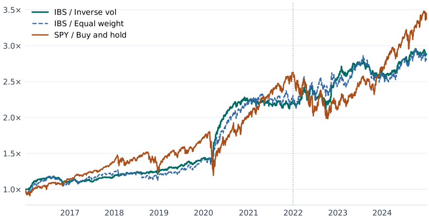
All three series start at 1. The dotted line marks the start of validation in 2022.
| 2016–2024 | Inverse-volatility IBS | Equal-weight IBS | Fully invested SPY |
|---|---|---|---|
| Annualized return | 12.51% | 12.21% | 14.47% |
| Cumulative return | +188.30% | +181.43% | +236.75% |
| Maximum drawdown | −12.93% | −12.97% | −33.79% |
| Sharpe | 1.32 | 0.91 | 0.86 |
| Average exposure | 43.55% | 65.71% | 100% |
Fully invested SPY earned the higher annualized return over the full period. Inverse-volatility IBS had a shallower drawdown and a higher Sharpe. In validation, the candidate earned 8.86% annualized and fully invested SPY earned 8.67%. The checker also scales SPY’s daily returns by the candidate’s average validation exposure (47.58%). This benchmark earned 4.43% annualized, leaving the candidate ahead by 4.43 percentage points.
SPY uses the same close-to-close price series as the project checker, with no trading costs deducted. Both IBS series include the backtest’s modeled trading costs.
Parameter sensitivity and candidate selection
The candidate’s maximum drawdown in validation was −12.9%. I tested eight neighboring configurations by varying the entry threshold, maximum holding period, volatility window, and position cap by ±20%, one at a time. Their validation Sharpes ranged from 0.609 to 0.977, all above the study’s 0.5 threshold. The main comparison captures the combined effect of changing the entry threshold, holding period, and weighting rule.
Another variant exited when IBS rose above 0.8 and recorded a validation Sharpe of 1.138. Round five’s predefined selection rule ranked passing strategies by training Sharpe, so the inverse-volatility version remained the primary candidate. Recording that rule makes it clear which results drove selection and which were used for validation.
What the results still leave open
The backtest computes IBS from the completed daily bar and assumes an execution at that same close. In live trading, market-on-close orders have to be submitted in advance. Price moves in the last few minutes can change the signal and the target weight, a timing issue the cost model does not capture.
Validation spans just three years. Repeated strategy screening, survivorship bias in the ETF universe, and shifting correlations across market regimes can all make development results look stronger. The research plan reserved 12 unseen instruments from January 2025 through November 2026 for a final holdout test. This article reports development and validation results. The project report gives no results for that holdout.
What would confirm alpha?
The next step is to freeze the selected file and score it on the independent holdout. Ralph gives me a reproducible set of candidates and failed experiments. The evidence for alpha still depends on how the frozen strategy performs on new instruments, a later period, and executable fills.
Project sources: the Strategy Lab round-five report, machine-readable check results, strategy implementations, and daily backtest engine.